Fuzzy zeros in percentile normalization

An important but potentially confusing aspect of our percentile normalization method to correct for batch effects is that we add noise to the zeros. I’ve gotten a few questions about this, and wanted to write this short blog post to illustrate why we did this and why it improves the method.

As a reminder, for each feature in a study, percentile normalization converts its abundances in control samples into a uniform distribution, and then converts the abundances in case samples to the percentile of the uniform that they fall on. In others words, the controls are a null distribution and cases are converted to values describing where they fall on the control distribution.

To convert control abundances into a uniform, we use SciPy’s percentileofscore function:

import scipy.stats as sp
sp.percentileofscore?

Signature: sp.percentileofscore(a, score, kind='rank')
Docstring:
The percentile rank of a score relative to a list of scores.

A `percentileofscore` of, for example, 80% means that 80% of the
scores in `a` are below the given score. In the case of gaps or
ties, the exact definition depends on the optional keyword, `kind`.

Parameters
----------
a : array_like
    Array of scores to which `score` is compared.
score : int or float
    Score that is compared to the elements in `a`.
kind : {'rank', 'weak', 'strict', 'mean'}, optional
    This optional parameter specifies the interpretation of the
    resulting score:

    - "rank": Average percentage ranking of score.  In case of
              multiple matches, average the percentage rankings of
              all matching scores.
    - "weak": This kind corresponds to the definition of a cumulative
              distribution function.  A percentileofscore of 80%
              means that 80% of values are less than or equal
              to the provided score.
    - "strict": Similar to "weak", except that only values that are
                strictly less than the given score are counted.
    - "mean": The average of the "weak" and "strict" scores, often used in
              testing.  See

              http://en.wikipedia.org/wiki/Percentile_rank

Returns
-------
pcos : float
    Percentile-position of score (0-100) relative to `a`.

For each feature in each case sample, we convert its abundance to a percentile rank of that feature’s abundances across all control samples. So if we start out with 10 control samples with the following abundances for a given feature: [0.1, 0.1, 0.2, 0.2, 0.3, 0.3] and we have a case sample with abundance 0.2, then it gets converted to 0.5, because 0.2 is in the 50th percent rank of the control distribution (in fact, it is the median value):

sp.percentileofscore([0.1, 0.1, 0.2, 0.2, 0.3, 0.3], 0.2, 'mean')
#Out[9]: 50.0

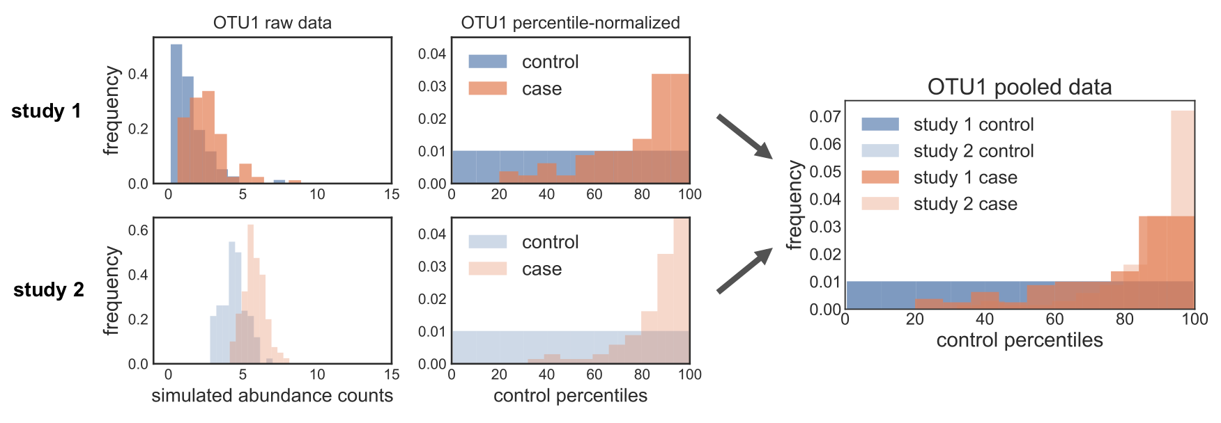
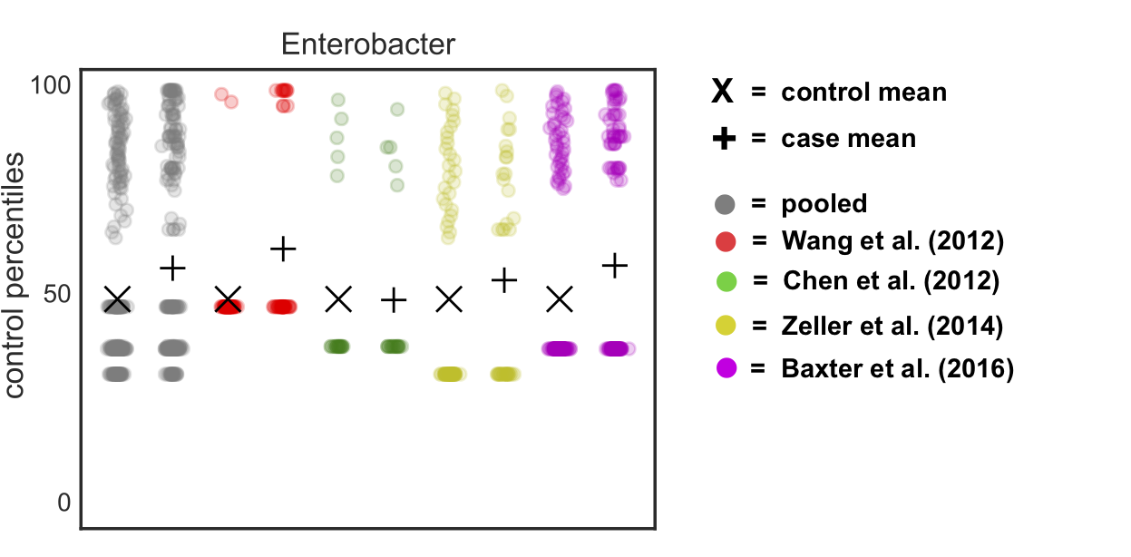
When we first started working on the method, we called this function straight on the relative abundances, without correcting for zeros. However, we noticed some weird behavior for more sparse OTUs: when we percentile normalized the data, we got a pile-up of values corresponding to zero abundance. The problem was that this rank pile-up wasn’t in the same place across studies, since it depends on what proportion of controls are zero, which is different in every study. So when we pooled the percentile normalized data, we noticed that these different rank pile-ups actually led to spurious associations driven by batch effects. In the figure below, you can see this clearly: the ranks pile up in different places across the different studies, and so pooling the data leads to data distributions that can mess up downstream non-parametric tests. Oh no!

The reason this is happening actually makes total sense, if you think about how the percentile normalization function is working. In our case, we’re calling it with the mean score: the value is converted to its rank in the provided array, and in cases of ties it is the mean rank of all those tied values. So if the first 50% of your data is zeros, then all of those zeros will be converted to 0.25, because 25% is the mean rank of the values that make up the first 50% of the data.

# Make a list with 5 zeros and 5 random numbers between 0 and 1
a = 5*[0.0] + list(np.random.uniform(0, 1, 5))

# Print a
print(', '.join(['{:.2f}'.format(i) for i in a]))
#0.00, 0.00, 0.00, 0.00, 0.00, 0.36, 0.97, 0.47, 0.11, 0.66

# Percentile normalize 0.0 with respect to a
sp.percentileofscore(a, 0.0, 'mean')
#Out[25]: 25.0

In other words, if zero is the first 20% of the cumulative distribution of your data, then the mean percentile rank of the value zero is 10%.

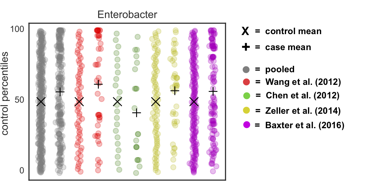
The way we got around this problem was by adding noise to the zeros, drawn randomly from a uniform going between 0 and something smaller than the smallest value. Thus, we convert all the zeros in the data to values that are different from each other (and thus won’t have the same rank), but which are less than the smallest non-zero number (and thus will have a lower rank than the “real” data).

If we go back to our previous example, where 0.11 is the lowest value, this would look like:

# Add noise to the zeros
a_fuzzy = [np.random.uniform(0, 0.01) if i == 0.0 else i for i in a]

# Print a
print(', '.join(['{:.3f}'.format(i) for i in a_fuzzy]))
#0.004, 0.006, 0.007, 0.006, 0.007, 0.360, 0.974, 0.471, 0.108, 0.659

# Check that this fixes the rank pile-up problem

## Percentile normalize 0.0 with respect to a
sp.percentileofscore(a_fuzzy, 0.0, 'mean')
#Out[33]: 0.0

## Percentile normalize a non-zero value with respect to a
sp.percentileofscore(a_fuzzy, 0.8, 'mean')
#Out[34]: 90.0

## Check that this non-zero values has the same percentile in the original data
sp.percentileofscore(a, 0.8, 'mean')
#Out[35]: 90.0

If we do this to our real data, we see two things: (1) the control distributions are now actually uniform (unlike before, where we saw the pile-up at the mean “zero” rank) and (2) we’ve gotten rid of the rank pile-ups in each study and the pooled data:

Theoretically speaking, we’re basically removing any claim on the informativeness of the value of zero in our data. All we know is that it is a smaller value than the smallest observed value, but we don’t know whether some of those zeros are “true” zeros (i.e. the organism is not present) vs. “false” zeros (i.e. the organism is present but unobserved). Thus, adding this noise is actually a fairly conservative thing to do. But it allows us to sleep at night and correct for batch effects - win win!